Build a Naïve and an Advanced RAG System – and Evaluate It

In the previous post, we laid the foundation of our RAG system. Based on the use case, we created a vector store, generated a synthetic test set, and defined the metrics we’ll use to evaluate performance. In this fifth part, we will build two pipelines: a simple naïve baseline and a more advanced extension. We will run both on our synthetic test set and compare them using the same metrics.

We model the pipeline as a graph via LangGraph: each node represents a step (e.g., retrieve, rerank, generate) and edges define control flow. Nodes are simple callables (e.g., LLM calls), and edges determine what runs next (fixed or conditional). This makes pipelines explicit, debuggable, and easy to extend. For a beginner-friendly overview, check out this.

Naïve RAG Pipeline

We keep the naïve pipeline as simple as possible and include only the three core RAG steps.

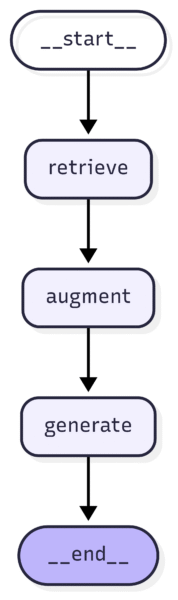
You can see the full naïve graph structure here.

At runtime, a user question triggers retrieval of the most relevant chunks from the vector store. Then, the retrieved context plus the user question are passed to the system prompt, and finally, the LLM generates an answer grounded in that context.

Advanced RAG System

Next, we extend the baseline with three retrieval-side upgrades before generation:

1. Query decomposition/expansion. An LLM proposes subqueries for complex prompts; we retrieve chunks for the original query and for each subquery.
2. Reciprocal Rank Fusion (RRF). We fuse the multiple result lists into one using a robust rank-fusion method.
3. Cross-encoder reranking. We rescore top candidates with a cross-encoder to improve the final ranking.

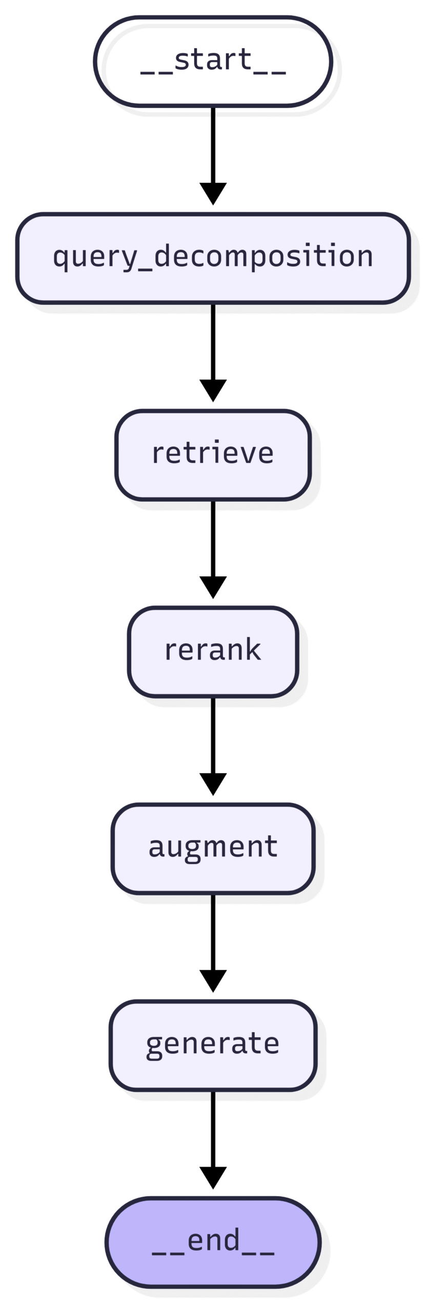
Again, check out here for the full graph structure of the advanced RAG graph.

Concretely, before the initial retrieval runs, a lightweight LLM decides whether the input is complex enough to warrant subqueries. If so, it generates additional subqueries based on the original question. Retrieval is then multi-stage: we retrieve for the original and each subquery. After retrieval, we first merge lists via RRF and then rerank with a cross-encoder. From that point on, the pipeline is identical to the baseline: we augment the (re-)ranked context with the original query and let the LLM generate an answer.

Evaluate the Pipeline

With both graphs defined, we can evaluate them.

We begin by configuring the graph: we choose the generative LLM, set the k parameter for retrieval, and specify how many answers to sample per query. We generate 3 answers per query to reduce variance. LLM outputs are stochastic, thus averaging metric scores across multiple samples yields more stable comparisons.

from src.graph.components.configuration import Configuration
from langchain_core.runnables import RunnableConfig

# choose the RAG graph you want to test
import src.graph.naive_rag as rag_graph # naïve rag pipeline
# OR
import src.graph.advanced_rag as rag_graph # advanced rag pipeline


# graph configuration 
cfg = Configuration(
    provider="anthropic", # choose the provider 
    answer_gen_model="claude-sonnet-4-20250514", # choose the LLM gen model
    top_k=10, # number of top document chunks to retrieve
    num_answers=3, # number of answers to generate 
)

run_cfg = RunnableConfig(
    configurable=cfg.model_dump()
    )

After configuration, we iterate over the synthetic questions, store the question, the retrieved context, and the generated answers, and additionally measure latency as a simple cost proxy. Finally, we compute the RAG triad metrics for each question. The helper `rate_dataset` runs the metrics asynchronously across items to speed things up.

# load the packages
import pandas as pd
import time
from tqdm import tqdm

# 1.) load synthetic data set
synth_data = pd.read_csv("data/synthetic_qa_pairs/synthetic_qa_pairs_filtered.csv")

results = []

# 2.) Iterate through the questions, retrieve context and generate answers
for idx in tqdm(range(len(synth_data)), desc=f"Generating Answer for Question..."):
    question = synth_data.iloc[idx]['input']
    
    try:
        # Run RAG pipeline
        start_time = time.time()
        result = rag_graph.graph.invoke(
            {"question": question}, 
            config=run_cfg
        )
        process_time = time.time() - start_time
        
        # Create base result dictionary
        result_dict = {
            'query_id': idx, # the query ID
            'question': question, # the query
            'gold_answer': synth_data.iloc[idx]['expected_output'], # the gold answer (we don't need it, but you can use it for your own eval)
            'latency': process_time, # processing time (how long does it take to get the answer?)
            'context': [ctx.page_content for ctx in result['context']], # the retrieved context chunks
        }
        
        # Add individual answers (if we generate more than 1)
        for ans_idx, answer in enumerate(result['answers'], 1):
            result_dict[f'answer_no_{ans_idx}'] = answer # each generated answer (in this case: 3)
        
        results.append(result_dict)
        
    except Exception as e:
        print(f"Error processing question {idx}: {str(e)}")
        continue

# 3.) Run the evaluation
from src.utils.evals import rate_dataset 

rated_results = asyncio.run(rate_dataset(results, model="gpt-4o-mini", max_concurrency=5))

That’s it! We ran each test question through the pipeline, captured retrieved contexts and answers, and computed the metrics for evaluation.

Comparing the Pipelines

We now compare the two systems. First, we load the saved outputs and use a small helper to compute means and standard errors across queries for each pipeline.

from src.utils.get_plots import get_stats_for_metrics 

# 1.) Load the saved outputs
file_list = [
    "results/simple_rag_res_rated.json", 
    "results/advanced_rag_res_rated.json"]

method_names = {
    file_list[0]: "naive RAG",
    file_list[1]: "advanced RAG",
}

# 2.) Compute query-level and overall summary statistics for each method
detailed_dfs, metrics_dfs = {}, {}

for fp in file_list:
    det, summ = get_stats_for_metrics(fp)
    label = method_names.get(fp, Path(fp).stem)
    detailed_dfs[label] = det
    metrics_dfs[label]  = summ

Then, we simply plot the results to get a visual read of the effect of the advanced techniques versus the baseline.

from src.utils.get_plots import plot_rag_metrics 

plot_rag_metrics(metrics_dfs, detailed_dfs)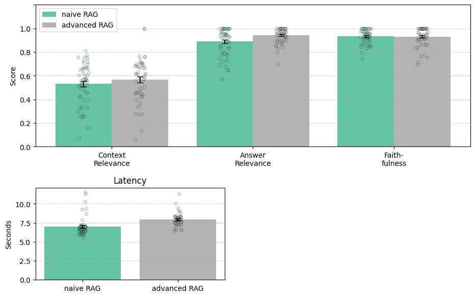

Key findings:

• Latency increases (by ~1 second), which is unsurprising given the extra steps we perform.
• Context Relevance and Answer Relevance improve, suggesting the retrieval-side upgrades help. But note that this is simply a visual inspection and does not imply any statistical significance.
• Faithfulness remains unaffected, implying that reranking does not modulate hallucination rates in our example.

What you see is a classic cost-benefit decision. If your use case tolerates ~1 s of additional latency for a notable increase in answer/context relevance, the advanced pipeline is attractive; if not, keep the baseline and optimize elsewhere.

In the next (and last) part of this series, we’ll take a closer look into our own RAG implementation at the Science Media Center. We will show additional statistics to illustrate how the improvements actually increased performance and look under the hood at what happens when users interact with the RAG bot.