After experimenting with many different techniques, we combined the most promising ones (i.e., those that showed performance improvements through visual inspection of the plots compared to the baseline model) and created an advanced RAG pipeline that is now used internally at the Science Media Center Germany.
First, we will explain the RAG system’s features. Then, we will show how those additional features affect performance through statistical tests. Finally, we will illustrate what happens under the hood when using the RAG bot.
Features of Our Pipeline
After testing several techniques, we found this approach showing the most promising results:
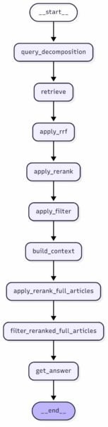
The first retrieval steps are analogous to the query decomposition and reranking technique that we showed in the previous post.
Specifically, when a user submits an initial query, a lightweight LLM first determines whether the query needs decomposition. If so, subqueries are generated. The retriever then retrieves the relevant text chunks for both the original query and the subqueries. The resulting retrieval lists are merged via Reciprocal Rank Fusion (RRF) and then reranked using a cross-encoder (we use this Cohere model, but feel free to use any cross-encoder model you have access to).
Essentially, a cross-encoder takes the input query and the retrieved text chunks and assigns a relevance score to each chunk, ranging from 0 to 1. In the next step, we remove all text chunks from the reranked top-k list of retrieved contexts that fall below a certain threshold. After testing different values, we set the threshold to 0.15, i.e., we remove all text chunks that have a relevance score lower than 15% as assigned by the reranking model.
So far, we have worked only with text chunks, i.e., pieces of text of fixed length. However, modern LLMs have such large context windows that we are no longer constrained by the input length. Thus, as the next step of the retrieval process, we use the retrieved chunks to fetch the full context. In other words, instead of using only the retrieved text chunk, we use the entire article in which the chunk appears. Note that this technique was mainly chosen because our stories are relatively short and mostly cover the same topic. If your knowledge base consists of very long documents covering different topics, this approach may be less useful than in our case.
Next, we use the cross-encoder again to assign relevance scores, but this time rating the entire article rather than just the chunk with respect to the query.
As the next step, we rerank our final list of retrieved articles once more. This time, we weight them by their release date, since we want answers to be grounded in more recent rather than older articles. To achieve this, we calculate a recency score that boosts newer articles over older ones. By combining both the relevance and recency scores, we obtain the final reranked context list.
Lastly, we forward the reranked list plus query to the system prompt and let the LLM generate an answer.
Statistical Findings
Before showing exactly what happens under the hood, let’s first look at how the combination of these techniques improves performance.
To test how the implemented features influenced performance, as measured via the RAG triad metrics, we applied a Bayesian linear regression model. Since this series is about RAG and not statistics, we won’t go into the statistical methods. (However, if you’re interested, feel free to read this.)
Also, we won’t get lost in the theoretical differences between frequentists and Bayesian statistics (there could be a whole blog series on this topic alone). For now, it’s enough to remember that the cool thing about Bayesian statistics is that it provides a posterior distribution, which directly quantifies our uncertainty about parameter values given the data. This makes interpretation more intuitive than frequentist p-values.
In simpler terms, when we want to test if feature A improves faithfulness (compared to baseline), Bayesian methods provide a distribution of plausible effect sizes. From this distribution, we can calculate the probability of direction, i.e., the probability that the effect is positive. For example, if 97% of the posterior distribution lies above zero, then there’s a 97% probability that feature A actually improved faithfulness. This direct probabilistic interpretation makes Bayesian approaches well suited for practical decision-making.
Now we can examine how our advanced RAG pipeline performs compared to the baseline. The plots show the posterior distributions for each advanced method’s effect on the RAG triad metrics relative to the baseline. The proportion of each distribution above zero indicates our confidence that the effect is positive. As a rule of thumb, when more than 95% of the posterior lies on one side of zero, this represents strong evidence for a directional effect.
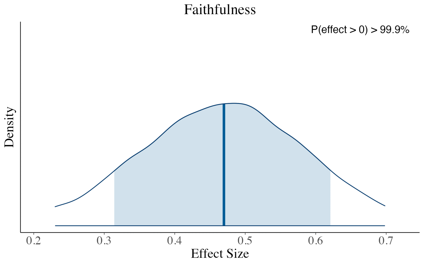
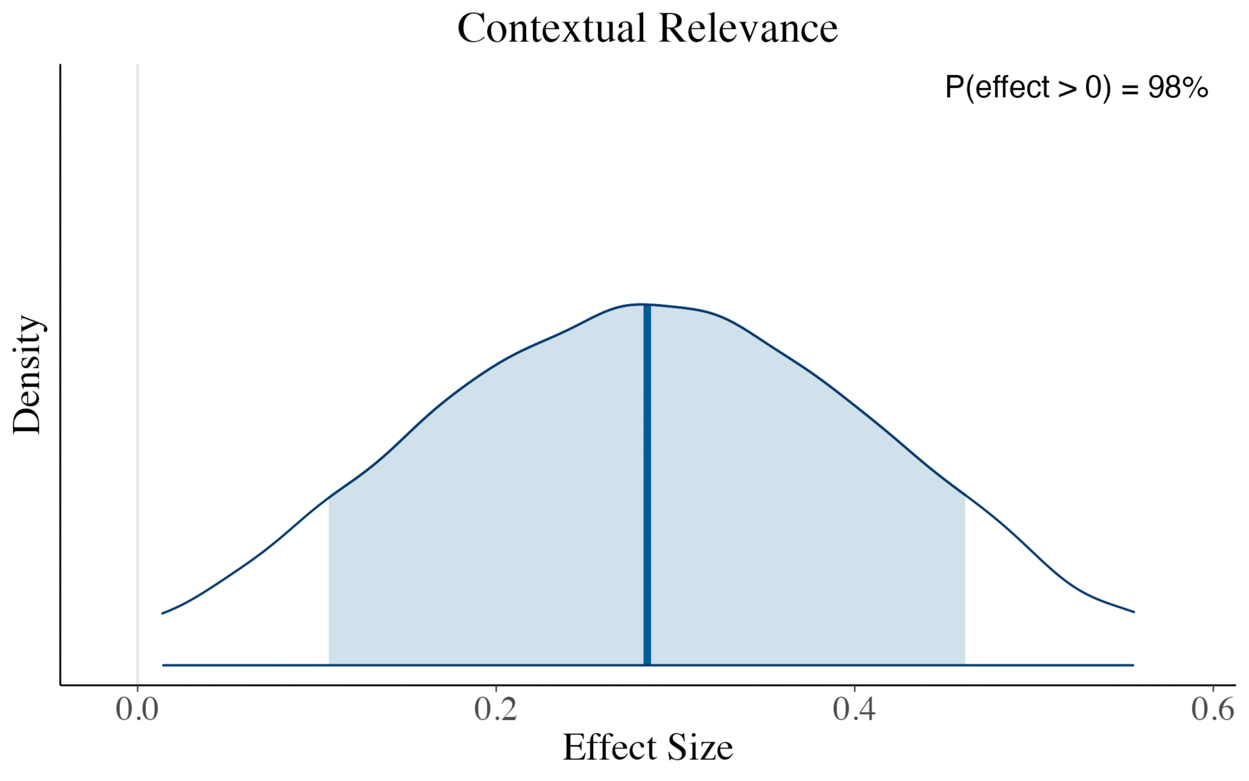
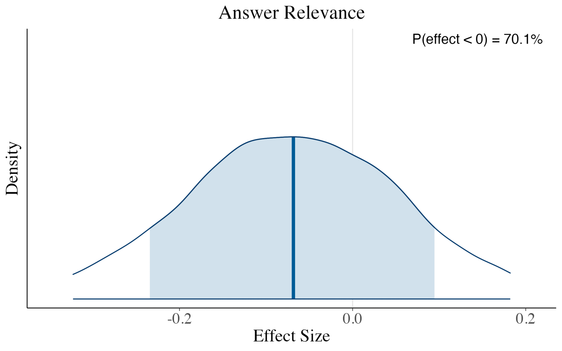
Key findings:
- We see a credible increase in Context Relevance and Faithfulness with our extended setup compared to the baseline (both values > 95%).
- Answer Relevance, however, is not credibly affected by the extension.
In practical terms, this means that our extensions help retrieve more relevant context for a query and ensure that the generated answers are better grounded in this context, i.e., lower rates of hallucination.
Our RAG Bot in Action
For internal use, we built our RAG bot with Streamlit and integrated it with LangSmith to enable full traceability of every step.
Demo Video
In the video, we submit the following query and hit enter:
An welchen Medikamenten zur Behandlung von Alzheimer wird derzeit geforscht, und wie wirken sie im Gehirn?
After ~25 seconds, the answer appears. The user can then:
- Expand the Source panel to see which passages support each quoted sentence in the answer.
- Switch to the Story Links tab to view the full documents (with links) used to produce the response.
Note: For our internal use, the relatively long response time is acceptable. The RAG bot mainly supports editorial research, where answer quality and reliability are far more important than speed. However, in user-centered scenarios, this may look different. Ultimately, it’s a trade-off, where you have to decide individually how to weigh latency against performance.
How it Works (Step by Step)
Under the hood, the following cascade of steps is triggered after hitting Enter:
Step 1 — Query decomposition
A lightweight classifier model decides whether the question is complex enough to decompose. Here it returns true, and a second model generates three subqueries (in addition to the original).Step 2 — Retrieval
For the original query plus the three subqueries (four in total), we run retrieval and return the top 10 text chunks for each query.Step 3 — RRF merge
We combine the four retrieval lists with RRF: duplicates are collapsed, and chunks that appear in multiple lists or rank higher in any list receive higher fused ranks.Step 4 — Cross-encoder rerank (chunk level)
The fused set contains 25 unique chunks. A cross-encoder reranks them and we keep the top 10.Step 5 — Post-hoc filter
We drop any chunk with a cross-encoder relevance score below 0.15, leaving only high-confidence evidence.Step 6 — Build context (document expansion)
Each chunk carries a Story ID in its metadata. We use these IDs to retrieve the full articles associated with the chunks. In this example, that yields seven full documents, since multiple chunks often come from the same article.Step 7 — Rerank again (document level)
We run the cross-encoder at the document level to score whole articles for relevance. Just like at the chunk level, we drop any articles with a relevance score below 0.15.Step 8 — Recency weighting
A simple decay function computes a recency score per article. We combine recency and relevance into a final score that determines the order of documents in the context window.Step 9 — Answer generation + transparent citations
We pass the initial query and the ranked context to the LLM to generate the answer. After generation, the model maps quoted sentences back to specific chunks, so users can verify claims. This is powered by Anthropic’s citations feature.
Next Steps
As you might remember from part 4 of our series, it’s best practice to use custom metrics tailored to the use case. As a next step, we plan to collect user feedback and use it as the basis for creating our own custom metrics, which we can then apply to further improve the system by combining user feedback with existing metrics and evaluation steps.
That’s it for our series. In the first three parts, we provided the theoretical background on RAG along with examples of how to use it. In the next two posts, we showed how to set up a simple RAG baseline, extend it, and then compare it qualitatively. In this final post, you saw how we implemented our own system at the Science Media Center Germany. The main purpose of this series was to give you a straightforward example of how to build your own RAG system and to demonstrate how metrics are useful not only for objectively measuring system performance but also for improving it through evaluation-driven feedback.