Now that we know why RAG is needed and how it helps to reduce the risk of hallucinations by compensating for the inherent limits of LLMs, we can take a closer look at how it actually works. In this series, we describe a RAG pipeline that can be broken down into four main stages: knowledge base creation, chunking, embeddings, and the actual RAG triad (i.e., retrieval-augmentation-generation steps). This breakdown reflects the approach we’re following throughout the blog series. However, keep in mind that RAG pipelines can be designed in different ways, with alternative techniques applied at various stages.
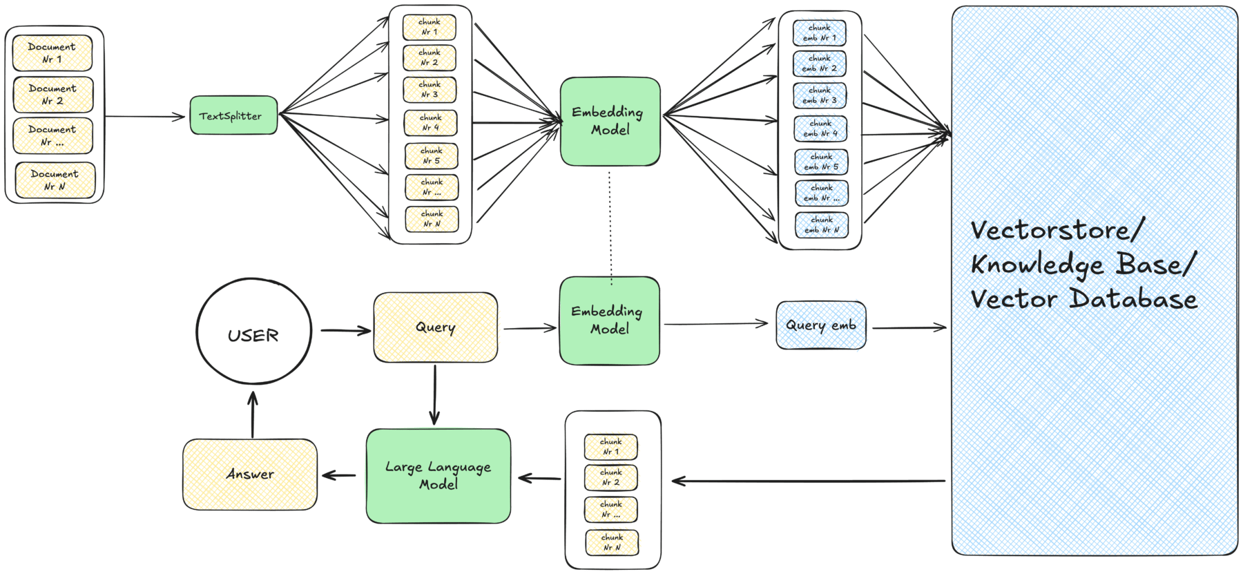
The diagram below shows the basic pipeline of such a system, which we will walk through step by step.
Knowledge Base
It all starts with the knowledge base. This is essentially a collection of text documents that we want the model to use as an additional source of truth. What matters here are two things: the content of the documents and their format.
Content-wise, the knowledge base might include internal reports, scientific articles, government documents, or even sensitive or leaked materials. In short, any material the model is unlikely to have seen during its original training.
Format-wise, these documents can appear as PDFs, plain text files, HTML pages, Word documents, or many other formats. Modern RAG frameworks can handle diverse file types, automatically extracting text content regardless of the original format.
The key idea is that the documents contain the information the LLM itself lacks, whether it’s time-sensitive material (e.g., recent developments not in the training data) or domain-specific material (e.g. internal reports, scientific publications, or legal texts).
Choosing the right knowledge base is crucial: if it is incomplete, outdated, or factually incorrect, even the best retrieval mechanism won’t help. This is why quality curation and regular updates of your knowledge base are essential.
Chunking
Instead of working with entire documents, we split them into smaller units called text chunks. Each chunk contains a limited amount of text, and we can define an overlap between consecutive chunks to avoid cutting important context at chunk boundaries.
Both the size of the chunks and the amount of overlap are parameters you can configure:
- Chunk size: The length of each piece (typically measured in tokens, but can also be characters or words).
- Chunk overlap: the amount of repeated text between two consecutive chunks (usually 10-20% of chunk size).
If chunks are too large, retrieval becomes imprecise. If they are too small, coherence is lost. Chunking ensures that the system can later retrieve exactly the part of a document that is most relevant to a query, rather than entire documents that might contain mostly irrelevant information.
Embeddings
Once we have chunks, we need to transform them into a format that a machine can work with. As mathematical models, LLMs do not operate directly on words, but on numerical representations. This is where embeddings come in. For example, the words “car” and “automobile” would have very similar embeddings because they have similar meanings, while “car” and “card” would have very different embeddings.
An embedding is a vector — i.e., a list of numbers — that captures the semantic meaning of a word, sentence, or passage.
To create embeddings, we use an embedding model (a specialized encoder trained on large amounts of text to understand semantic relationships). After converting all our chunks to embeddings, we store them in a vector database (or vector store). This database is optimized for fast similarity search: given an input, it can quickly find the chunks whose embeddings are closest in meaning.
At this point, our knowledge base has been indexed. Instead of a set of documents, we now have a searchable semantic map of their contents that enables meaning-based rather than keyword-based search.
The RAG triad: Retrieval, Augmentation, Generation
With the knowledge base indexed in the vector store, the RAG process itself begins when a user asks a question. This triggers the RAG triad:
1. Retrieval
The query is also converted into an embedding, using the same embedding model. The retriever then searches the vector store for the top-k most similar chunks using techniques like cosine similarity or dot product.
(Note: k here is simply the number of passages we want to return. This can be defined in the parameter settings.)
2. Augmentation
The retrieved chunks are combined with the user’s original query and fed into the LLM. This step augments the model’s system prompt (the default instruction we give the model to guide its behavior) with additional context.
A typical augmented prompt might look like:
You are a helpful assistant. Answer the user’s question based only on the provided context.
This is the question: [User’s original question]
Answer the question based on this context: [Retrieved Context]
3. Generation
The LLM then generates an answer grounded in the retrieved context, rather than relying only on its world knowledge from the frozen training data.
(Note: If you want to know more about how semantic similarity works (i.e., how comparing embeddings allows the system to identify semantically related text passages), you can find a nice explanation here.)
Summary
RAG works essentially by turning static documents into a dynamic, searchable knowledge base. This source is used to supply relevant context to an LLM in real time. The four stages described above – knowledge base creation, chunking, embeddings, and the RAG triad – form the backbone of this approach.
In the next post, we will look at how RAG can be applied in the context of science and data journalism and what motivated us at the Science Media Center to implement our own RAG tool.